This is just a sample topic...
Edit me
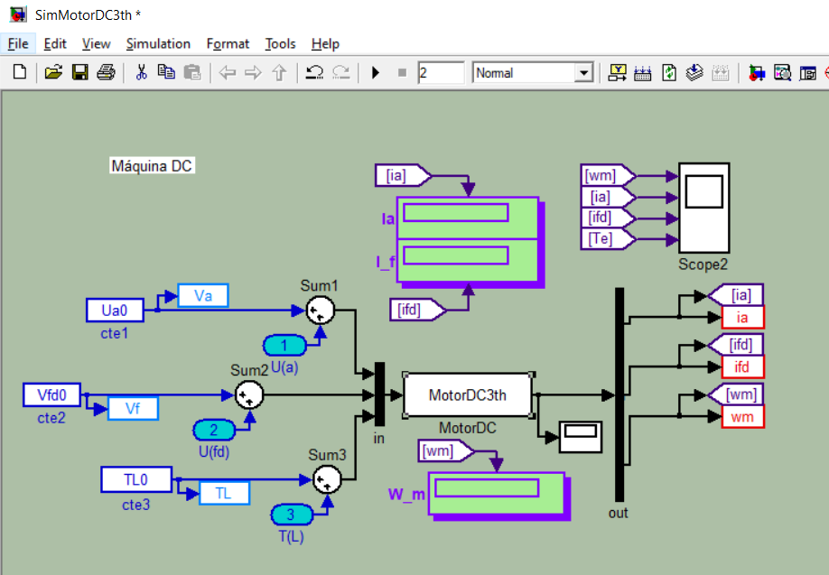
Simulación del motor DC
En este apartado se explica el proceso de inicialización de la máquina. En la figura se presenta la captura de pantalla del modelo realizado en simulink
dir=D:\wk_matlab\uc3m\mt\pc104\MTLB\src\Motors\DCmtr\mdl\3th_v2\rev1
Datos del motor
%% update 2021
% Datos dc motor conected separately excited

clear all; close all; clc
%{
Snom => rated power      [VA]        p =>   pair of poles
f    => rated frequency  [Hz]
Vll  => peak value of rated phase voltage [V]
1) Datos de placa del motor de cd
n -> velocidad [rpm]                        Ua -> Tensión en el inducido [V]
Ia -> intensidad en el inducido [A]    Vfd -> Tensión en el inductor [V]
ifd -> intensidad en el inductor [A]    P -> potencia [W]
wbase -> velocidad [rad/s]
%}
Pnom=2200;    n=1000;       Ua=220;     wbase=2*pi*n/60;
Vfd=200;         ia=11;          ifd=0.9;
%{
2) Circuito Electrico
Ra -> Resistencia de armadura [ohms]        La -> Inductancia de armadura [Henry]
Rf -> Resistencia de campo [ohms]            Lf -> Inductancia de campo [Henry]
J ->    [Kg/m^2]                B -> [Nms^2]    Kb ->   [Nm/A^2]
%d.Ra=8+1.4+3.8;     d.La=1;    d.Rf=350;  d.Lf=7.6;
... NOTA: Ea2=n2*Ea1/n1=208.727;    k_phi2=Ea2/w2=0.83397;
%}
d.Ra=2.442176945;  d.La=0.14098873;  d.Rf=211.5859;   d.Lf=7.1278;
d.J=0.01347;        d.B=0.006316;   d.Kb=1.909;

ini=[11; 0.9;104.7198]; TL0=20.33759;
save d
Modelado dinámico del motor de DC
%% update 2021
%{
 Simulation of DC Machine Transient Behavior
inputs  -> [Ua Uf  Tl]
states -> [ia if wm]
%}
function [sys,x0,str,ts]=MotorDC3th(t,x,u,flag,d,ini)
switch flag,
case 0,  [sys,x0,str,ts]=mdlInitializeSizes(d,ini);
case 1,  sys=mdlDerivatives(t,x,u,d);
case 3,  sys=mdlOutputs(t,x,u,d);
case {2,4,9},   sys=[];
otherwise
        error(['Unhandled flag=',num2str(flag)]);
end

function [sys,x0,str,ts]=mdlInitializeSizes(d,ini)
 sizes = simsizes;                  sizes.NumContStates  =3;
 sizes.NumDiscStates  =0;    sizes.NumOutputs     =3;
 sizes.NumInputs      =3;       sizes.DirFeedthrough =0;
 sizes.NumSampleTimes =1;   sys = simsizes(sizes);
x0=ini;     str=[];      ts=[0 0];

function sys=mdlDerivatives(t,x,u,d)
%Laf=d.Kb/ifd; %Te=Laf*ia*ifd;
Ua=u(1); Ufd=u(2); Tm=u(3);
ia=x(1); ifd=x(2); w=x(3);
dia=(Ua-d.Ra*ia-d.Kb*w)/d.La;
difd=(Ufd-d.Rf*ifd)/d.Lf;
Te=d.Kb*ia;
dw=(Te-d.B*w-Tm)/d.J;
sys=[dia;difd;dw];

function sys=mdlOutputs(t,x,u,d)
sys=[x(1);x(2);x(3)];
Inicialización del motor
%% update 2021
% datos del motor

TL0 = 0;    Ua0=0;  Vfd0=0;      % Note: These parameters must be zero
wmec0 = 1000*2*pi/60;  ia0=11; ifd0=0.9;
%wmec0 = 700*2*pi/60;  ia0=0.69; ifd0=0.9;
%wmec0 = 295*2*pi/60;  ia0=0.78; ifd0=0.9;
%wmec0 = 295*2*pi/60;  ia0=0.69; ifd0=0.9;
%i0=0.48 0.52 0.57 0.61 0.65 0.68 0.69 0.71 0.73 0.74 0.75 0.76 0.77 0.78 0.78 0.78 0.78 0.79 0.8 0.81 0.82 0.83

disp(sprintf('\t 1).  Operating Point Specifics Define '));
disp(sprintf('\t \t \t- wmec0  = %d  [rad/s]',wmec0));
disp(sprintf('\t  Unknown: '));
disp(sprintf('\t \t \t \t \t Ua, Vfd, Tm0 \n'));
NameModel='SimMotorDC3th';
Model_spec = operspec(NameModel) ; % obtiene el punto de operacion
... outputs
NameBlockOutAdd='SimMotorDC3th/out';
Model_spec=addoutputspec(Model_spec,NameBlockOutAdd,1);
Model_spec=addoutputspec(Model_spec,NameBlockOutAdd,2);
Model_spec=addoutputspec(Model_spec,NameBlockOutAdd,3);
... inputs
Model_spec.States(1).Known= [1 1 1]';           Model_spec.States(1).x = [ia0 ifd0 wmec0]';
Model_spec.Input(1).Known = 0;           Model_spec.Input(1).u = Ua0; %
Model_spec.Input(2).Known = 0;           Model_spec.Input(2).u = Vfd0; %
Model_spec.Input(3).Known = 0;           Model_spec.Input(3).u = TL0; %

Model_spec.Outputs(1).Known =1;                 Model_spec.Outputs(1).y     = ia0;
Model_spec.Outputs(2).Known =1;                 Model_spec.Outputs(2).y     = ifd0;
Model_spec.Outputs(3).Known =1;                 Model_spec.Outputs(3).y     = wmec0;
... Find the operating point values  about the operating point
[NameModel_op,op_report]=findop(NameModel,Model_spec);
ini=NameModel_op.States.x;                  Ua0 = NameModel_op.Input(1).u;
Vfd0 = NameModel_op.Input(2).u;         TL0 = NameModel_op.Input(3).u;
save NameModel_op
disp '¬¬¬¬¬¬¬¬¬¬¬¬¬¬¬¬¬¬¬¬¬¬¬¬¬¬¬¬¬¬¬¬¬¬¬¬¬';
disp(sprintf(' SOLUTION:'));            disp(sprintf(' Ua0  =%d',Ua0));
disp(sprintf(' Vfd0  =%d',Vfd0));      disp(sprintf(' TL =%d',TL0));
disp '¬¬¬¬¬¬¬¬¬¬¬¬¬¬¬¬¬¬¬¬¬¬¬¬¬¬¬¬¬¬¬¬¬¬¬¬¬';
salida al ejecutar el código
>> IniCond_2021
	 1).  Operating Point Specifics Define
	 	 	- wmec0  = 1.047198e+02  [rad/s]
	  Unknown:
	 	 	 	 	 Ua, Vfd, Tm0


 Operating Point Search Report:
---------------------------------

 Operating Report for the Model SimMotorDC3th.
 (Time-Varying Components Evaluated at time t=0)

Operating point specifications were successfully met.
States:
----------
(1.) SimMotorDC3th/MotorDC
      x:            11      dx:     -1.41e-12 (0)
      x:           0.9      dx:             0 (0)
      x:           105      dx:     -5.28e-13 (0)

Inputs:
----------
(1.) SimMotorDC3th/U(a)
      u:           227    [-Inf Inf]
(2.) SimMotorDC3th/U(fd)
      u:           190    [-Inf Inf]
(3.) SimMotorDC3th/T(L)
      u:          20.3    [-Inf Inf]

Outputs:
----------
(1.) SimMotorDC3th/out
      y:            11    (11)
(2.) SimMotorDC3th/out
      y:           0.9    (0.9)
(3.) SimMotorDC3th/out
      y:           105    (105)

¬¬¬¬¬¬¬¬¬¬¬¬¬¬¬¬¬¬¬¬¬¬¬¬¬¬¬¬¬¬¬¬¬¬¬¬¬
 SOLUTION:
 Ua0  =2.267740e+02
 Vfd0  =1.904273e+02
 TL =2.033759e+01
¬¬¬¬¬¬¬¬¬¬¬¬¬¬¬¬¬¬¬¬¬¬¬¬¬¬¬¬¬¬¬¬¬¬¬¬¬
Linealización del modelo
%% update 2021
% datos del motor

TL0 = 0;    Ua0=0;  Vfd0=0;      % Note: These parameters must be zero
wmec0 = 1000*2*pi/60;  ia0=11; ifd0=0.9;
%wmec0 = 700*2*pi/60;  ia0=0.69; ifd0=0.9;
%wmec0 = 295*2*pi/60;  ia0=0.78; ifd0=0.9;
%wmec0 = 295*2*pi/60;  ia0=0.69; ifd0=0.9;
%i0=0.48 0.52 0.57 0.61 0.65 0.68 0.69 0.71 0.73 0.74 0.75 0.76 0.77 0.78 0.78 0.78 0.78 0.79 0.8 0.81 0.82 0.83

disp(sprintf('\t 1).  Operating Point Specifics Define '));
disp(sprintf('\t \t \t- wmec0  = %d  [rad/s]',wmec0));
disp(sprintf('\t  Unknown: '));
disp(sprintf('\t \t \t \t \t Ua, Vfd, Tm0 \n'));
NameModel='SimMotorDC3th';
Model_spec = operspec(NameModel) ; % obtiene el punto de operacion
... outputs
NameBlockOutAdd='SimMotorDC3th/out';
Model_spec=addoutputspec(Model_spec,NameBlockOutAdd,1);
Model_spec=addoutputspec(Model_spec,NameBlockOutAdd,2);
Model_spec=addoutputspec(Model_spec,NameBlockOutAdd,3);
... inputs
Model_spec.States(1).Known= [1 1 1]';           Model_spec.States(1).x = [ia0 ifd0 wmec0]';
Model_spec.Input(1).Known = 0;           Model_spec.Input(1).u = Ua0; %
Model_spec.Input(2).Known = 0;           Model_spec.Input(2).u = Vfd0; %
Model_spec.Input(3).Known = 0;           Model_spec.Input(3).u = TL0; %

Model_spec.Outputs(1).Known =1;                 Model_spec.Outputs(1).y     = ia0;
Model_spec.Outputs(2).Known =1;                 Model_spec.Outputs(2).y     = ifd0;
Model_spec.Outputs(3).Known =1;                 Model_spec.Outputs(3).y     = wmec0;
... Find the operating point values  about the operating point
[NameModel_op,op_report]=findop(NameModel,Model_spec);
ini=NameModel_op.States.x;                  Ua0 = NameModel_op.Input(1).u;
Vfd0 = NameModel_op.Input(2).u;         TL0 = NameModel_op.Input(3).u;
save NameModel_op
disp '¬¬¬¬¬¬¬¬¬¬¬¬¬¬¬¬¬¬¬¬¬¬¬¬¬¬¬¬¬¬¬¬¬¬¬¬¬';
disp(sprintf(' SOLUTION:'));            disp(sprintf(' Ua0  =%d',Ua0));
disp(sprintf(' Vfd0  =%d',Vfd0));      disp(sprintf(' TL =%d',TL0));
disp '¬¬¬¬¬¬¬¬¬¬¬¬¬¬¬¬¬¬¬¬¬¬¬¬¬¬¬¬¬¬¬¬¬¬¬¬¬';
Determinación de la función de transferencia
load NameModel_tf
%{
DH=step([num_tf{i,j}],[den_tf{i,j}],t)  specify the transfer function from input j to output i
%}
clc
... separacion de los terminos de tf
[num,den]=tfdata(NameModel_tf);  %celldisp(num);celldisp(den)
... Funciones de transferencia obtenidas:
...NUM{i,j} and DEN{i,j} specify the  transfer function from input j to output i.
tf11=NameModel_tf(1,1);  %(i,j)  Ua &ia
tf31=NameModel_tf(3,1);  %(i,j)  Ua &wm
tf22=NameModel_tf(2,2);  %(i,j)  Ufd &ifd
tf13=NameModel_tf(1,3);  %(i,j)  Tm &ia
tf33=NameModel_tf(3,3);  %(i,j)  Tm &wm

disp '¬¬¬¬¬¬¬¬¬¬¬¬¬¬¬¬¬'
disp('control Ufd & ifd')
[A22,B22,D22,H22]=tf2ss(num{2,2},den{2,2}); printsys(A22,B22,D22,H22) %
... comportamiento en lazo abierto
figure('Name',' disturbance step response to Ifd')
t=[0:0.001:0.5];  [y,x,t]=step(num{2,2},den{2,2},t); % respuesta al escalon
subplot(3,1,1),plot(t,y);grid; xlabel('Time [sec]'); ylabel('ifd [N]'); hold on
[P,Z]=pzmap(num{2,2},den{2,2})
... Comportamiento en lazo cerrado
...figure('Name','Close-loop disturbance step response')
[num_cl,den_cl]=cloop(num{2,2},den{2,2});
roots(den_cl) % para conocer los polos inestables %[r,k]=rlocfind(tf_cl);
[y,x,t]=step(num_cl,den_cl,t); % respuesta al escalon
subplot(3,1,2),plot(t,y);grid; xlabel('Time [sec]'); ylabel('ifd [sec]'); hold on
... controlador PI
...figure('Name','Close-loop with control')
tf_ctr22=tf(13693*[0.019 1],[1 0]);  save tf_ctr22
...figure(1), bode (tf_ctr35);  figure(2),
... nyquist (tf_ctr35) %That's the Im-axis in the Nyquist diagram
tf_ctrOK=series(tf_ctr22,tf22);     tf_cl=feedback(tf_ctrOK,1);
[y,x]=step(tf_cl,t);
subplot(3,1,3),plot(t,y); xlabel('time [sec]'), ylabel('ifd(t)')
Ajuste del control
NOTA: revisar esta con los chicos
D:\wk_matlab\uc3m\mt\pc104\MTLB\src\Motors\DCmtr\mdl\3th_v2\rev5
Directorios Motor DC
Modelado matemático del motor dc
Diseño del control del motor de dc
pc104\MTLB\src\Motors\DCmtr\mdl\3th_v2\rev5
pc104\MTLB\bin\MyComputePrg
parte de modelado del motor
pc104\MTLB\src\Motors
Implementación del control con PSIM
dir=D:\wk_matlab\uc3m\mt\pc104\Matlab\basics\goals\REDUCTOR\buck_with_dc_machine
Implementación experimental del motor con XPCtarget
dir=D:\wk_matlab\uc3m\mt\pc104\Matlab\basics\goals\REDUCTOR\xpctarget
[]: