This is just a sample topic...
Edit me
Sample Content
Code Repo = D:\wk_matlab\uc3m\mt\pc104\Matlab\ElctPtc\inversor\inversor3ph
VSC & STATCOM,
Se resuelve en sistema en representación ODE definiendo el solver mas adecuado
Code Repo = D:\wk_matlab\uc3m\mt\pc103\MTLB\CTR\solveODE
clear all; close all; clc

Vll=30; fnom=50;  d.L=10e-3;       d.R=3.5;
Udc=300;
%% valores a por unidad
Vbase=Vll*sqrt(2/3);
ibase=2*sqrt(2);
Sbase=(3/2)*ibase*Vbase;
%Zbase=Vbase/ibase; Lbase=Zbase/wbase; Cbase=1/(Zbase*wbase);
d.wbase=2*pi*fnom;
S=complex(5e1,2e1);  U=complex(30*sqrt(2/3),0);
I=(2/3)*conj(S/U);   id0=real(I); iq0=imag(I);

%% usando ODE
%%
tspan=[0 0.2];	Xo=[id0 iq0];
Dd=0.01 ;  Dq=0;  Vd=300*Dd; Vq=300*Dq;
dVd=real(U)-Vd ,   dVq=imag(U)-Vq

%id=x(1), iq=x(2)
%fA=inline('[(d.L*d.wbase*x(2) - d.R*x(1) + dVd )/d.L ;(-d.L*d.wbase*x(1)- d.R*x(2) + dVq )/d.L]');
%invtrSMALLsgn=@(t,x)[fA];

invtrSMALLsgn=@(t,x)...
		[(d.L*d.wbase*x(2) - d.R*x(1) + dVd )/d.L;...
		 (-d.L*d.wbase*x(1)- d.R*x(2) + dVq )/d.L];

[t,y]=ode45(invtrSMALLsgn, tspan, Xo);
iDQ0=y(end,:), plot(t,y);
pause(2); close all
Repaso de control
Code Repo = D:\wk_matlab\uc3m\mt\pc103\MTLB\CTR\Xian
Análisis de la respuesta del sistema de control
Code Repo = D:\wk_matlab\uc3m\mt\pc103\MTLB\statcom\dgrmBLCK
Modelado & Setting completo
Code Repo = D:\wk_matlab\uc3m\mt\pc104\Matlab\ElctPtc\MODELS_STATCOM_ck\KaiSimMdl
clear all; close all; clc

%% simbolicEQ
%{
syms L u R t w
%e=u+CUR*complex(R,L*w)
%w=sym('w(t)');tht=diff(w,t)
tht=int(w,t)
CUR=sym('CUR(t)')
euler=exp(-j*tht);
CUR=CUR*euler
U_L=L*diff(CUR,t)
U_R=CUR*R
Ug=u*exp(-j*tht)
break
%}

d=struct('R',24.8e-3,'L',2e-3,'w',100*pi);
s=tf('s');
[aD,aFF]=deal(d.L*s+d.R,d.L*d.w);
M=[aD,-aFF;aFF,aD];%M=[d.L*s+d.R,-d.L*d.w;d.L*d.w,d.L*s+d.R];
Madj=[aD aFF;-aFF aD];
detM=aD*aD-(-aFF*aFF);
invM=Madj/detM;

tf1=aD/detM;
tf2=aFF/detM;
G_jw=[0 tf(-aFF);tf(aFF) 0]

fprintf('\n*************************\n')
Gbis=minreal(invM/(1-(Madj*G_jw/detM)))

GJW=feedback(invM,G_jw,1)

t=0:0.1:10; dltU=-0.1*(t>4 & t<6);%disturbance
u=[ones(size(t));ones(size(t))];%u=[Vd;ones(size(t))];
%lsimplot(GJW,u,t)

G=1/M;
set(G,'InputName',{'id','iq'},'OutputName',{'Vd','Vq'},'variable','p');
fprintf('sysFT: Gzpk')

Gzpk=zpk(minreal(G));%Gzero=tzero(G);
Gss=ss(Gzpk);fprintf('sysSS: Gss')
[sysG1,g,T,Ti]=balreal(minreal(Gss))
%type='modal';%companion
%[G1,T]=canon(G,type);%balreal(G1)%minreal(G)
G2ss=ss2ss(sysG1,T)
%H=[0 -d.L*d.w;d.L*d.w 0];
Gdscpl=minreal(feedback(G,G_jw,1))

F=(d.R/d.L)*eye(2);
F=[0 -1;1 0]
G_=(1/d.L)*eye(2);
%dotX=

kFF1=1/dcgain(G(2,1)); kFF2=1/dcgain(G(1,2));
C1=tf(kFF1,[1 0]);     C2=tf(kFF2,[1 0]);
kC=[0 kFF1;kFF2 0];    cl_ff=G_*kC

%'InputName',{'w_ref','Td'},'OutputName','w'
%set(cl_ff);

%title('Setpoint tracking and disturbance rejection')
% Annotate plot
%line([5,5],[.2,.3]); line([10,10],[.2,.3]);
%text(7.5,.25,{'disturbance','T_d = -0.1Nm'},...
 %           'vertic','middle','horiz','center','color','r');

%% FEEDBACKctr
%rlocusplot
Grlc=Gdscpl;
sysRLCS=tf(1,[1 0])*Grlc(1,1);
[R,K] = rlocus(sysRLCS)


TFp=tf(1,[1 d.L/d.R]);
[R,K] = rlocus(tf(1,[1 0])*TFp)
for idx=1:1:length(K)%-13
%KK=K(10);
KK=K(idx)
CC=tf(KK,[1 0])
GCL=feedback(CC*TFp,1)
%rlocusplot(GCL); hold on
stepplot(GCL);hold on
end

ctrC=append(CC,CC)
figure();G_FB=feedback(ctrC*Grlc,1,1,1);
step(G_FB,2);

%figure();lsimplot(cl_ff,G_FB,u,t);
%set(G_FB,'InputName',{'uq','ud'},'OutputName',{'id','iq'});
%title('Setpoint tracking and disturbance rejection')
%legend('feedforward','feedback w/ rlocus','Location','NorthWest')

figure();bodeplot(cl_ff,G_FB)
Bibliografia:
- Kai tesis dinamarca
- TFM Linda & Barrado
Modelo promediado
dir
`D:\wk_matlab\uc3m\mt\pc104\MTLB\src\ElctPtc\MODELS_STATCOM_ck\statcomFiltro`
Co-simulación con PSIM
D:\wk_matlab\uc3m\mt\pc104\MTLB\src\ElctPtc\MODELS_STATCOM_ck\statcom_plots_thesis_danesa\inversor\inversor3ph\myCodeInverter3ph_work
Actualización del modelo de un inversor promediado
Descripción de la planta (modelo dinámico)
%% x=[id iq Vd Vq Idc] u=[Vdc f Dd Dq]     parameters => [L C R]   inputs: outputs:
function [sys,x0,str,ts] = inv3ph(t,x,u,flag,d,ini)
switch flag,
    case 0,  [sys,x0,str,ts]=mdlInitializeSizes(d,ini);
    case 1,  sys=mdlDerivatives(t,x,u,d);
    case 3,  sys=mdlOutputs(t,x,u,d);
   case { 2, 4, 9 },         sys = [];
    otherwise,    error(['Unhandled flag = ',num2str(flag)]);
end

function [sys,x0,str,ts]=mdlInitializeSizes(d,ini)
sizes = simsizes;     sizes.NumContStates=4;     sizes.NumDiscStates=0;
sizes.NumOutputs=5;     sizes.NumInputs=4;     sizes.DirFeedthrough=1;
sizes.NumSampleTimes=1;  sys=simsizes(sizes);     x0=ini;      str=[];       ts=[0 0];

function sys=mdlDerivatives(t,x,u,d)
... u=[Vdc f Dd Dq]
Vdc=u(1);   f=u(2); Dd=u(3); Dq=u(4);
id=x(1); iq=x(2); Vd=x(3); Vq=x(4);
omega=2*pi*f;
did=Dd/(3*d.L)*Vdc+omega*iq-Vd/(3*d.L);
diq=Dq/(3*d.L)*Vdc-omega*id-Vq/(3*d.L);
dVd=(id/d.C)+omega*Vq-(Vd/(d.R*d.C));
dVq=(iq/d.C)-omega*Vd-(Vq/(d.R*d.C));
sys=[did;diq;dVd;dVq];

function sys=mdlOutputs(t,x,u,d)
Vdc=u(1);   f=u(2); Dd=u(3); Dq=u(4);
id=x(1); iq=x(2); Vd=x(3); Vq=x(4);
Idc=Dd*id+Dq*iq;
sys=[id;iq;Vd;Vq;Idc];
Inicialización
... Ecuaciones Carlos Alvarez
addpath('D:\wk_matlab\uc3m\mt\pc104\Matlab\MyComputePrg\inverter3ph');
addpath('D:\wk_matlab\uc3m\mt\pc104\Matlab\MyComputePrg\ctr');

%% Load datas
addpath('D:\wk_matlab\uc3m\mt\pc104\Matlab\DataSheet'); dtInverter3ph_v2

%% normalizar datos
%{
d.R=R/Zbase; d.L=L/Lbase; %d.C=1/(C/Cbase);% pud.omega=wbase; %pu
C_base=pi^2/(3*Zbase); d.C=C/C_base; Udc_base=3*Vll/pi;
Vdc0=Udc/Udc_base
%}

 %d.R=R;  d.L=L; d.C=C;  save d

Vdc0=450;   theta_inv=0;
%theta_inv=0;
Vd0=Vbase*cos(theta_inv)/sqrt(2);  Vq0=Vbase*sin(theta_inv)/sqrt(2);
%% inicialization
Idc0=4;  frec0=50;   id0=-1.95;  iq0=-0.05;
ini=[id0;iq0;Vd0;Vq0]; Dd0=0; Dq0=0;

disp 'Operating Point Specs:';
disp(sprintf('%s=%d','id0',id0,'iq0',iq0,'Vd0',Vd0,'Vq0',Vq0,'Idc0',Idc0));
disp 'Unknown: Dd0, Dq0';

NameModel='SimInv3ph'; NameModel_spec = operspec(NameModel);  % find operating point
% outputs
NameOutputAdd1='SimInv3ph/outC';
NameModel_spec=addoutputspec(NameModel_spec,NameOutputAdd1,1); %id
NameModel_spec=addoutputspec(NameModel_spec,NameOutputAdd1,2); %iq
NameModel_spec=addoutputspec(NameModel_spec,NameOutputAdd1,3); %Vd
NameModel_spec=addoutputspec(NameModel_spec,NameOutputAdd1,4); %Vq
NameModel_spec=addoutputspec(NameModel_spec,NameOutputAdd1,5); %Id
% inputs
NameModel_spec.Input(1).Known=1;    NameModel_spec.Input(1).u=0;  %Vdc0
NameModel_spec.Input(2).Known=1;    NameModel_spec.Input(2).u=0;  %frec
NameModel_spec.Input(3).Known=0;    NameModel_spec.Input(3).u=Dd0;  %Dd0
NameModel_spec.Input(4).Known=0;    NameModel_spec.Input(4).u=Dq0;  %Dq0
% states      .....   1-know 0-unknow
NameModel_spec.States.Known=[0 0 1 1]'; NameModel_spec.States.x=[id0 iq0 Vd0 Vq0]';
%[Idc0 I2dc0]
NameModel_spec.Outputs(1).Known=0;  NameModel_spec.Outputs(1).y= id0;
NameModel_spec.Outputs(2).Known=0;  NameModel_spec.Outputs(2).y=iq0;
NameModel_spec.Outputs(3).Known=1;  NameModel_spec.Outputs(3).y= Vd0;
NameModel_spec.Outputs(4).Known=1;  NameModel_spec.Outputs(4).y=Vq0;
NameModel_spec.Outputs(5).Known=0;  NameModel_spec.Outputs(5).y= Idc0;
%}
% calculate operating point specific
[NameModel_op,op_report]=findop(NameModel,NameModel_spec);
ini=NameModel_op.States.x;
Dd0= NameModel_op.Input(3).u; Dq0 = NameModel_op.Input(4).u;
disp '-- Solution: ---------';
disp(sprintf('%s=%d \t','Dd0',Dd0,'Dq0',Dq0));
save NameModel_op


%% linealizacion
NameInput1='SimInv3ph/Sum3'; NameModel_io(1)=linio(NameInput1,1,'in'); %Dd
NameInput2='SimInv3ph/Sum4'; NameModel_io(2)=linio(NameInput2,1,'in'); %Dq
%NameOutputAdd1='SimInv3ph/outC';
NameModel_io(3)=linio(NameOutputAdd1,3,'out');    NameModel_io(3).OpenLoop='on';
NameModel_io(4)=linio(NameOutputAdd1,4,'out');    NameModel_io(4).OpenLoop='on';

setlinio(NameModel,NameModel_io);
NameModel_lin=linearize(NameModel,NameModel_op,NameModel_io);
set(NameModel_lin,'inputn',{'Dd';'Dd'},'outputn',{'Vd';'Vq'},'statename',{'Id';'Iq';'Vd';'Vq'});

%save('.\ctr_mtx\NameModel_lin2');
NameModel_io(1)=linio(NameInput1,1,'none');
NameModel_io(2)=linio(NameInput2,1,'none');
NameModel_io(3)=linio(NameOutputAdd1,3,'none');   NameModel_io(3).OpenLoop='off';
NameModel_io(4)=linio(NameOutputAdd1,4,'none');   NameModel_io(4).OpenLoop='off';
setlinio(NameModel,NameModel_io); size(NameModel_lin);
NameModel_tf=tf(NameModel_lin);% save('.\ctr_mtx\NameModel_tf2');
NameModel_can= canon(NameModel_lin,'modal');%forma canonica
NameModel_tf_can=tf(NameModel_can);

%% makeCtrs

[numtf,dentf]=tfdata(NameModel_tf);  %save('.\ctr_mtx\numtf2');  save('.\ctr_mtx\dentf2');
Gs=NameModel_tf(1:2,1:2); [numGs,denGs]=tfdata(Gs);
Gs_det=minreal(Gs(1,1)*Gs(2,2)-(Gs(1,2)*Gs(2,1))); %det_A=a11*a22-a12*a21;
Gs_adj=[Gs(2,2) -Gs(2,1);-Gs(1,2) Gs(1,1)];%adjunta
Gs_inv=minreal(mldivide(Gs_det,Gs_adj));%%invA=minreal(mldivide(det_A,adj_A))
X_s=eye(2);
Ds=minreal(mtimes(Gs_inv,X_s)); %%Ds=minreal(mldivide(Gs,X_s))
Qs=minreal(mtimes(Ds,Gs));
D12=minreal(mrdivide(-Gs(1,2),Gs(1,1)));D21=minreal(mrdivide(-Gs(2,1),Gs(2,2)));
D_s=[1 D12;D21 1], [numD_s,denD_s]=tfdata(D_s);
%save('.\ctr_mtx\numD_s2'); save('.\ctr_mtx\denD_s2')
Qs=minreal(mtimes(D_s,Gs)), [numQs,denQs]=tfdata(Qs);
Q11=minreal(Gs(1,1)*(1-(minreal((Gs(1,2)*Gs(2,1))/(Gs(1,1)*Gs(2,2))))));
Q22=minreal(Gs(2,2)*(1-(minreal((Gs(1,2)*Gs(2,1))/(Gs(1,1)*Gs(2,2))))));
num_C4=10.61*[0.0011 1];  den_C4=[1 0];C4=tf(num_C4,den_C4);
num_C5=10.61*[0.0011 1];  den_C5=[1 0]; C5=tf(num_C5,den_C5);
Ctr2=[C4 1;1 C5]; [numCtr2,denCtr2]=tfdata(Ctr2);
%save('.\ctr_mtx\numCtr2');     save('.\ctr_mtx\denCtr2');
%}N
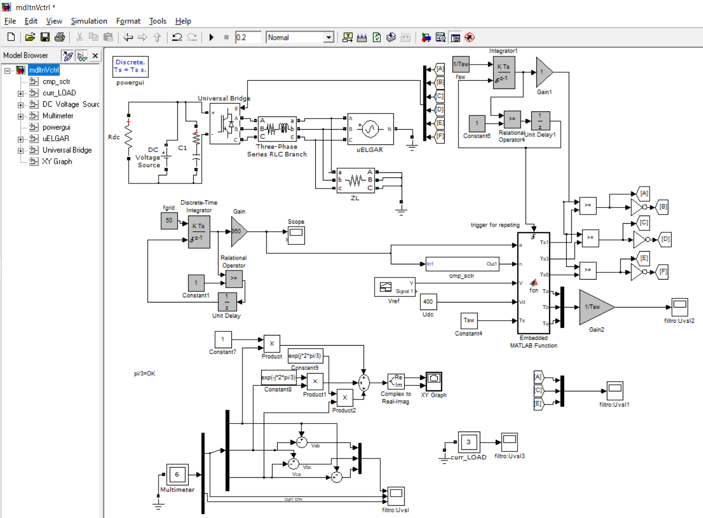
Esquematico de simulación de planta
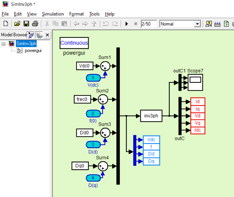
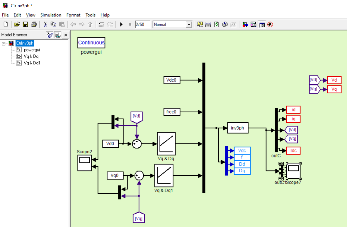
Esquematico de simulación de planta con control
Salida de inicialización en workspace
Operating Point Specs:
id0=-1.950000e+00iq0=-5.000000e-02Vd0=1.327906e+02Vq0=0Idc0=4
Unknown: Dd0, Dq0


Operating Point Search Report:
---------------------------------

 Operating Report for the Model SimInv3ph.
 (Time-Varying Components Evaluated at time t=0)

Operating point specifications were successfully met.
States:
----------
(1.) SimInv3ph/S-Function1
      x:      1.33e+03      dx:     -3.64e-12 (0)
      x:          1.25      dx:             0 (0)
      x:           133      dx:             0 (0)
      x:             0      dx:             0 (0)

Inputs:
----------
(1.) SimInv3ph/V(dc)
      u:             0
(2.) SimInv3ph/f(0)
      u:             0
(3.) SimInv3ph/D(d)
      u:          0.29    [-Inf Inf]
(4.) SimInv3ph/D(q)
      u:          5.56    [-Inf Inf]

Outputs:
----------
(1.) SimInv3ph/outC
      y:      1.33e+03    [-Inf Inf]
(2.) SimInv3ph/outC
      y:          1.25    [-Inf Inf]
(3.) SimInv3ph/outC
      y:           133    (133)
(4.) SimInv3ph/outC
      y:             0    (0)
(5.) SimInv3ph/outC
      y:           392    [-Inf Inf]

-- Solution: ---------
Dd0=2.898478e-01 	Dq0=5.562318e+00


State-space model with 2 outputs, 2 inputs, and 4 states.

D_s =

  From input "Vq" to output...
   Vd:  1

            628.3 s + 1.047e08
   Vq:  ---------------------------
        s^2 + 3.333e05 s + 5.457e06

  From input "Vd" to output...
            -628.3 s - 1.047e08
   Vd:  ---------------------------
        s^2 + 3.333e05 s + 5.457e06

   Vq:  1

Continuous-time transfer function.


Qs =

  From input "Dd" to output...
                   2.5e09 s^4 + 3.333e15 s^3 + 1.667e21 s^2 + 3.703e26 s + 3.086e31
   Vd:  ---------------------------------------------------------------------------------------
        s^6 + 1.667e06 s^5 + 1.111e12 s^4 + 3.703e17 s^3 + 6.172e22 s^2 + 4.115e27 s + 6.736e28


        -24.37 s^7 + 7.498e08 s^6 + 6.364e14 s^5 + 1.708e20 s^4 + 1.428e25 s^3 + 1.911e27 s^2

                                                                          + 1.46e30 s + 1.404e32

   Vq:  ----------------------------------------------------------------------------------------

        s^10 + 1.667e06 s^9 + 1.111e12 s^8 + 3.704e17 s^7 + 6.175e22 s^6 + 4.119e27 s^5

                             + 3.54e29 s^4 + 8.241e32 s^3 + 4.117e34 s^2 + 4.076e37 s + 6.598e38


  From input "Dd" to output...

        -24.37 s^7 + 1.789e08 s^6 + 1.607e14 s^5 + 4.388e19 s^4 + 3.706e24 s^3 + 1.373e27 s^2

                                                                         + 4.081e29 s + 1.233e32

   Vd:  ----------------------------------------------------------------------------------------

        s^10 + 1.667e06 s^9 + 1.111e12 s^8 + 3.704e17 s^7 + 6.175e22 s^6 + 4.119e27 s^5

                             + 3.54e29 s^4 + 8.241e32 s^3 + 4.117e34 s^2 + 4.076e37 s + 6.598e38


                   2.5e09 s^4 + 3.333e15 s^3 + 1.667e21 s^2 + 3.703e26 s + 3.086e31
   Vq:  ---------------------------------------------------------------------------------------
        s^6 + 1.667e06 s^5 + 1.111e12 s^4 + 3.703e17 s^3 + 6.172e22 s^2 + 4.115e27 s + 6.736e28

Continuous-time transfer function.
SOURCE: D:\wk_matlab\uc3m\mt\pc104\MTLB\src\ElctPtc\MODELS_STATCOM_ck\statcom_plots_thesis_danesa\inversor\inversor3ph\DQ_new\rev1
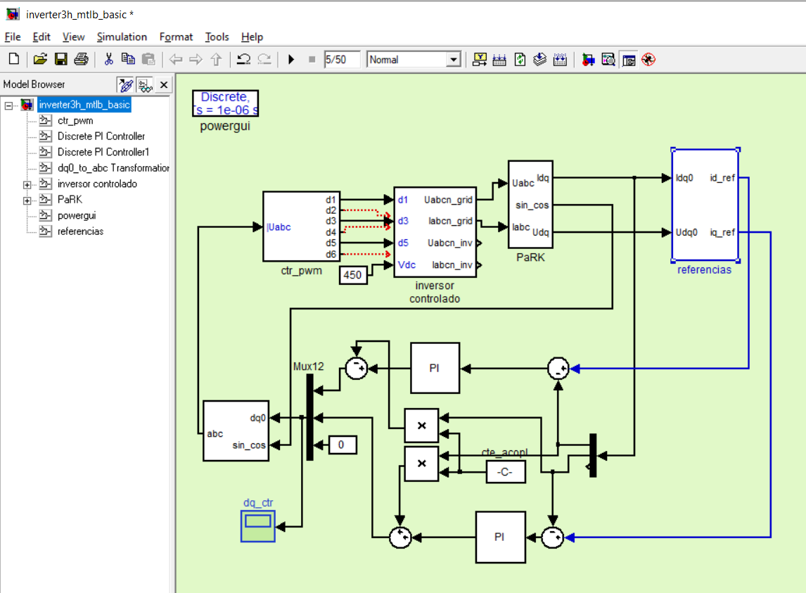
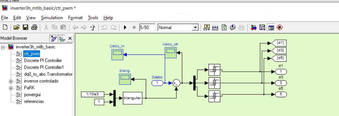
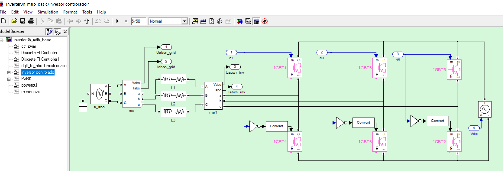
Implementación del inversor con matlab (modelo similar al de PSIM)
SOURCE:D:\wk_matlab\uc3m\mt\pc104\MTLB\src\ElctPtc\MODELS_STATCOM_ck\statcom_plots_thesis_danesa\inversor\inversor3ph\DQ_new\test_19Nov2011
Modulación vectorial implementación en Matlab
function [Ts1,Ts3,Ts5,Ta,Tb,To] = fcn(a,n,V,Vd,Ts)
%{
INPUTS:
a-> angle
n-> number of sectors
V-> (2/3)Vdc or less
Vd-> Vdc
Ts-> switching time

OUTPUTS:
Ts1-> time of switches
Ts3->
Ts5->
%}
%#eml

a=a.*pi./180;%degree2radian
s=(3.^0.5).*(V/Vd).*Ts;
Ta= s.*sin((n.*pi./3)-a-pi./3);
Tb= s.*sin(a-(n-1).*pi./3);
To=Ts-Ta-Tb;%%To_off
Ts1=0;
Ts3=0;
Ts5=0;

switch n
    case 1
        Ts1= (Ts-(Ta+Tb+To./2))./Ts;         Ts3= (Ts-(Tb+To./2))./Ts;       Ts5= (Ts-(To./2))./Ts;
    case 2
         Ts1= (Ts-(Ta+To./2))./Ts;         Ts3= (Ts-(Ta+Tb+To./2))./Ts;      Ts5= (Ts-(To./2))./Ts;
    case 3
        Ts1= (Ts-(To./2))./Ts;         Ts3=(Ts-(Ta+Tb+To./2))./Ts;         Ts5=  (Ts-(Tb+To./2))./Ts;
    case 4
        Ts1= (Ts-(To./2))./Ts;         Ts3=(Ts-(Ta+To./2))./Ts;     Ts5= (Ts-(Ta+Tb+To./2))./Ts;
    case 5
        Ts1= (Ts-(Tb+To./2))./Ts;         Ts3= (Ts-(To./2))./Ts;      Ts5=(Ts-(Ta+Tb+To./2))./Ts;
    case 6
         Ts1=(Ts-(Ta+Tb+To./2))./Ts;          Ts3= (Ts-(To./2))./Ts;      Ts5= (Ts-(Ta+To./2))./Ts;
end
return;
source:D:\wk_matlab\uc3m\mt\pc104\MTLB\src\ElctPtc\modulation